Using HTML and CSS to view Types in the JHS platform of J

Time flies when you are having fun, or maybe just time flies as I look back to how long it is since I have posted here. In any case I am back and ready to explore some new developments in the way that I am using the JHS platform of J.

One of the things that has frustrated me with J is that at times I spend a lot of time trying to figure out problems based on simple (and incorrect) assumptions I have about the information that I am being shown. J has an elegantly minimalistic way of showing the results of operations in its interactive environment. Unfortunately, it does not always distinguish between certain key qualities when it displays its results. It becomes my job as a programmer to confirm what I am seeing as what is really being presented and this is especially true for type information. With modern web browsers it has become possible to provide this additional information as part of the results and this is explored in the following video.

Since there was not enough time to go into all the details the screens below provide some of the background to the css and elements of html that are created in order to provide the new html based display. I provide this information for all to use and only ask that if you use it that in your best judgement you use it in a mindfully positive way.

Types

I hope to follow up in a week with the HTML and CSS approaches I have explored to display differently shaped arrays unambiguously, but last time I said that resulted in almost two years between posts. 🙂

Augmented View of Arrays (Redux)

Follow-up:

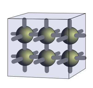
After looking back at the previous post I did notice one mistake. The shape for the following diagram should have been 1 2 3 instead of 2 3. If the shape had been 2 3 then the diagram would have had a plane rather than a cube as the ‘shape structure’.

 1 2 3 $ 0

Augmenting Frank’s Dual-View Representation by Simplifying:

After several weeks of reflection, I realized that the previous solution to visualizing Frank’s Dual-View could be made simpler  by displaying the absence of edges when there are zero valued dimensions in the shape. The following post will compare the two options with a following critique of the differences.

Case 0 – Empty shape for scalar value – Shape ’empty’

 

Old version

New version

Critique: The only difference here is colour to distinguish the two approaches as we move forward. Remember that scalar values in J do not have a shape of 0, but instead have a shape that is an empty list. Since there is no 0 in an empty list there is no change in representation of scalars.

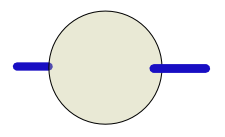
Case 1 – A list of zero items – Shape 0

 

Old version

New version

Critique: Both versions have the axle indicating that this is a list and that items can be added. Both versions are also greyed out as a visual cue that this is an empty list. The new version shows that the dimension that is zero is along the x axis (the only axis, as indicated by the axle) and so this is an empty list, as opposed to an empty matrix or cube which we will see later. Even though this adds an element in the visualization of an empty array, it will provide a more simple representation of non-empty arrays.

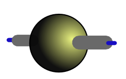
Case 2 – A list of one item – Shape 1

 

Old version

New version

Critique: This is where the advantage of the new approach starts to appear. Instead of the extra horizontal line, only the line presenting the one dimensional shape is included. The colour indicates that the shape is non-zero immediately.

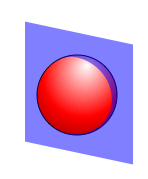
Case 3 – A matrix of one item – Shape 1 1

 

Old version

New version

Critique: The advantage continues as the plane immediately indicates the two dimensional shape and the single sphere indicates only one item. No extra lines required for the vast majority of arrays which are non-empty.

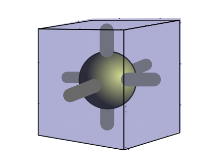
Case 4 – A cube of one item – Shape 1 1 1

 

Old version

New version

Critique: Again we have a single atom and the surrounding cube indicates three dimensions. The extra edges in the previous version are not required which really cleans up the display

Case 5 – A matrix of one item – Shape 0, Shape 0 1, and Shape 1, 0

 

Shape 0

Shape 0 1

Shape 1 0

Critique: The displays of these three empty arrays show that the one dimensional and two dimensional are clearly distinguishable, as is the difference between Shape 0 1 and Shape 1 0 matrices.

Case 6 – A cube of shape 1 2 3

 

Old version

New version

Critique: The spacing of the spheres easily shows the shape of the array and the enclosing cube outline immediately shows that the array has a three dimensional shape. If it were two dimensions the spheres would be embedded in a two dimensional plane. Again no more and no less than what is required to differentiate and describe the shape.

Case 7 – A cube of shape 0 2 3

Critique: This one was thrown in to show how a zero value in the leading axis of a three dimensional array would look. There are two rows and three columns of zero items which is why the spheres are greyed out with a front facing zero mark on the z axis. Contrast this with the 1 2 3 shape described in the preceding example.

Case 8 – A cube of shape 2 2 3

 

Old version

New version

Critique: I think that I may want to play around with the spacing on this one as this is one case where the new representation actually seems more confusing than the old version. Part of it may be the inherent structure that the extra edges provide, but I think this can be made up by using the spacing to reveal the relationships between the spheres as rows and columns. The text version of J uses this spacing to great effect, so I feel I am moving the right direction even though this version feels relatively unorganized.

In closing:

This time I promise; the next post will look at the representation of higher ranked arrays. I was happy to spend the extra time revising the display, as the higher dimensional representations really benefit from the cleaner look.  Until next time, I look forward to any feedback you may have.

Augmenting the Dual-View Array Representation

Follow Up:

My previous post included a verb to facilitate visualization of the Dual-View representation by returning coefficients representing array components:

   arrayCoeff =: +//.@(*/)/@,.&1

Unfortunately, this verb fails for scalars because it can’t deal with the empty list shape of rank 0 arrays.

   arrayCoeff ''
|domain error: arrayCoeff
|       arrayCoeff ''

A better solution has the array itself as the argument, then determines its shape and triggers an exception when dealing with scalars.

   arrayCoeffS =: +//.@(*/)/@,.&1`1:@.(''&-:)@$

where

 (''&-: )@$

returns 1 for a scalar argument.

   arrayCoeffS 4  NB. Scalar, array rank 0, shape ''
1
   arrayCoeffS 3 $ 4 NB. Vector, array rank 1, shape 3
3 1
   arrayCoeffS 2 3 $ 4 NB. Matrix, array rank 2, shape 2 3
6 5 1

Augmenting Frank’s Dual-View Representation:

This will allow arrays of shape 0 and shape 0 1 to be shown as distinct.
The Dual-View shows these shapes as identical because rank 2 can’t be represented by a single edge.

   arrayCoeffS 0$0 NB. Empty list of rank 1
0 1 

   arrayCoeffS 0 1$0 NB. No list of length 1 (rank 2)
0 1 1

Clearly they differ in the rank 2 array’s planar component, and changing the orientation of the single edge to indicate the plane is identical to the result of:

   arrayCoeffS 1 0$0 NB. One list of length 0 (rank 2)
0 1 1 

The way forward is to display the rank of the array even when the zero valued axes are not present. With distinguishable ranks, rank 1 and 2 arrays will be distinct. For rank 0 (scalar), the representation is the disk alone.

   arrayCoeffS 2 NB. Scalar value of 2 (rank 0)
1 

Arrays of rank 1 have a horizontal line through the disk indicating that the list can add items either before or after the value. If the shape is 0, only this rank line is shown with an empty value – a greyed out disk.

A non-zero axis uses thicker edges with rank line extended.

Rank 2 arrays indicate rank as an x-y plane encompassing the disk, allowing axes indication without affecting rank representation.

With rank 3 the embedding structure is a cube, with potential axes in three dimensions.

By including the rank information the augmented Dual-View shows previously indistinguishable arrays distinctly:

   0$0 

   0 1 $ 0 

   1 0 $ 0 

While typical arrays display as expected.

   2 3 $ 0 

   2 2 3 $ 0 

In the next post I will look at the representation of higher ranked arrays. Until then, I look forward to any feedback you may have.