An update on the Jig visuals

A couple of changes based on valuable feedback by Raul Miller and David Leibs and a quick note based on a comment by John Baker.

First the note: I should be clear that Jig at this point is not a working prototype but is in a design phase. It seems to me that there are three distinct aspects to this development. The design of the output is what I have focussed on here, but as well there is the generation of the information to create that output and the actual execution that will display the output. I am using Keynote in this design phase and will be moving back into the other two phases when I feel that the output is adequately defined. The next step will be using J to create the information needed using display foreigns 5!:1 and 5!: 6 for order of execution and and container level as well as type foreigns to indicate the appropriate colouring and shading of the nodes/containers. The second step will be to convert this information into an SVG element that will display the visual within a JHS environment.

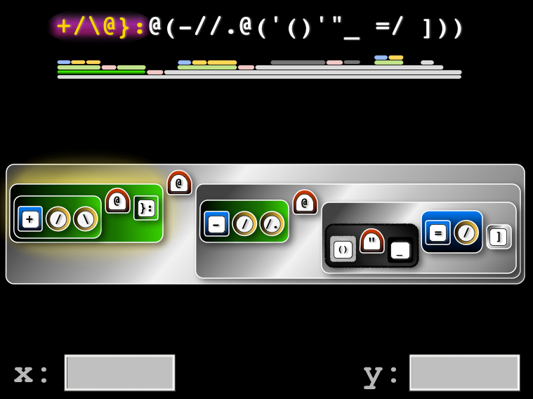
JigContainerAmbiPrevious visual display of ambivalent verb in Jig


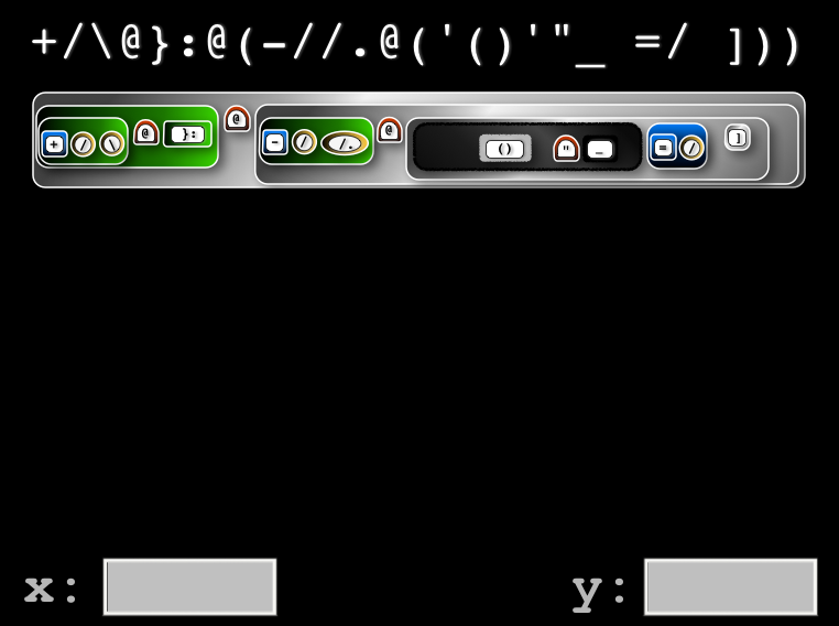
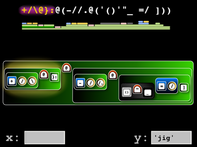
Screen Shot 2014-08-09 at 10.55.55 AMNew visual display of ambivalent verb in Jig

Based on the feedback of Raul and David, it became clear that although the topographic version would contain the necessary information, it may not display in as accessible a manner (specifically the fact that it was colour driven and that it is difficult to accommodate shading differences on that scale). David suggested more inline on the set container and by reducing the sizes I can still retain the correspondence with the sentence. Longer sentences would need to be accommodated by sliders to move the window or by zooming. That is in the display execution layer, but I think it is achievable.

For now I am happier with the results and look forward to more comments for further refinement.

Jig – a way of looking at J

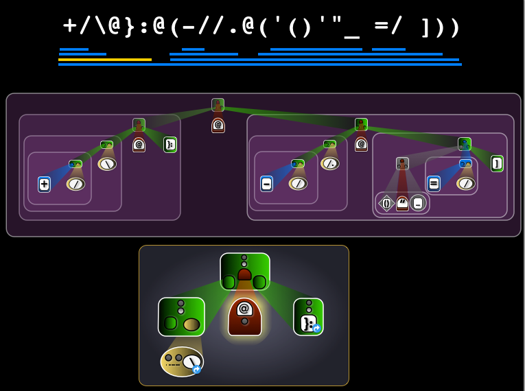
Initially, I had created a tree type view of J sentences. The sentence that I used was +/\@}:@(-//.@('()'"_ =/ ])), a monadic verb that returns the depth of a parenthesized sentence. It had enough complexity that it gave me a chance to see if the representation could handle some of the curves that this sentence threw at it. It could. The text box at the top is where the editing takes place and the resulting tree changes with each change to the sentence. Once the sentence is in place the tree gives an opportunity to click on different parts that then provide a zoomed in view to look at specific input and output  values for the part of the tree selected. The topographic representation under the sentence also allows the different parts of the sentence to be selected. The downside of this is that the tree representation takes up too much space and actually requires more nodes than are necessary to show the structure.

Jigtree


Tree view of the J sentence


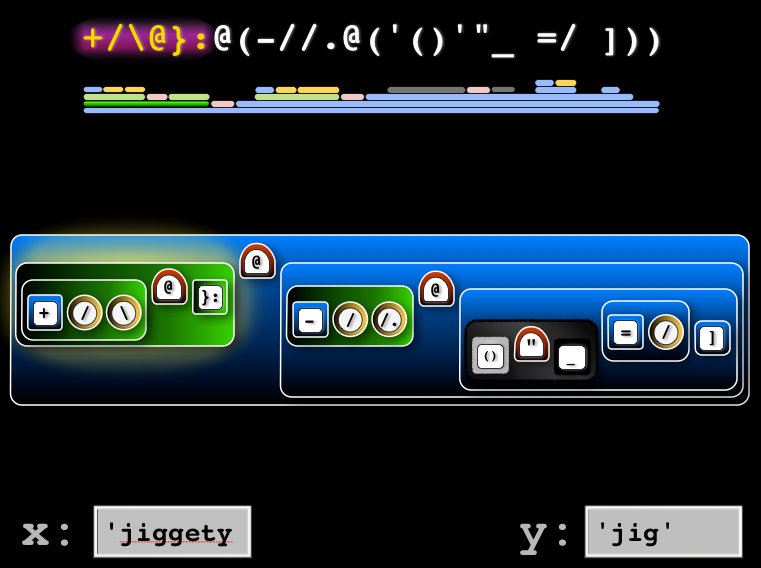
The next option is based on nested set containers that are able to retain the structure of the tree with reduced complexity. This also allows the display itself to function as the zoomed in portion so that there is more space for the entry of the x and y arguments. The result in this case is three different representations depending on whether the resulting verb is monadic, dyadic or has yet to have its arguments set (ambivalent). It also has the topographic representation that lines up with the sentence. Downside is that it is still a bit complex and seems to have some distance between the meaning of the sentence and its representation. The topographic view also has colours that correspond to the types of speech for the operators. This is noticeable as the colours change between monadic, dyadic and ambivalent instances.

JigContainerAmbi

Set container view of J sentence with no arguments set (ambivalent)


JigContainerDyadic

Set container view of J sentence with two arguments (dyadic).

JigcontainerMonadic

Set container view of J sentence with one argument (monadic).

It was during the process of developing the set container versions that I realized that the more graphic views of set container and tree display were not really providing any information that the topographic view did not also contain. Additionally, the topographic display has a correspondence to the original sentence that provides a stronger sense of connection to the structure for the observer. An additional idea that has not yet been developed is that there could be a slider that allows the sentence evaluation advance step by step as the sentence is parsed. The fact that the structure is not quite so visual when in topographic also gives the observer a bit more latitude in considering the temporal in addition to the spacial components of the sentence execution.

JigtopoDyadic

Topographic view of J sentence with two arguments (dyadic).

JigtopoMonadic

Topographic view of J sentence with one argument (monadic).

JigtopoAmbi

Topographic view of J sentence with no arguments set (ambivalent).

As a preview of coming events, it is my intention to develop this a little further using SVG for the topographic display and then having the inputs and outputs of each component of the partial result showing up as the different areas are clicked or as the slider progresses through the parsing of the sentence. Comments as always are welcome and future posts will likely trace the issues that arise as this design is implemented.

A Demo of ‘Extended’ Labs

In this post I am going to show a video of what can be done with the addition of media to labs (and that media includes parallel interfaces), but before that an overview of how these features are being put into place.


To begin, text files with .ijt extensions are recognized as lab files. The have a two part structure with the first part up to the single right parenthesis being the ‘lecture’, followed by text executed as if it were part of the operating environment. The results of this evaluation and the instructions are shown to the learner with one exception – the text preceded and followed by the PREPARE keyword is executed but neither they nor the results they produce are shown. This allows side effects such as having files loaded and run to adjust the environment and showcase specific concepts to be taught.


BlogLab1

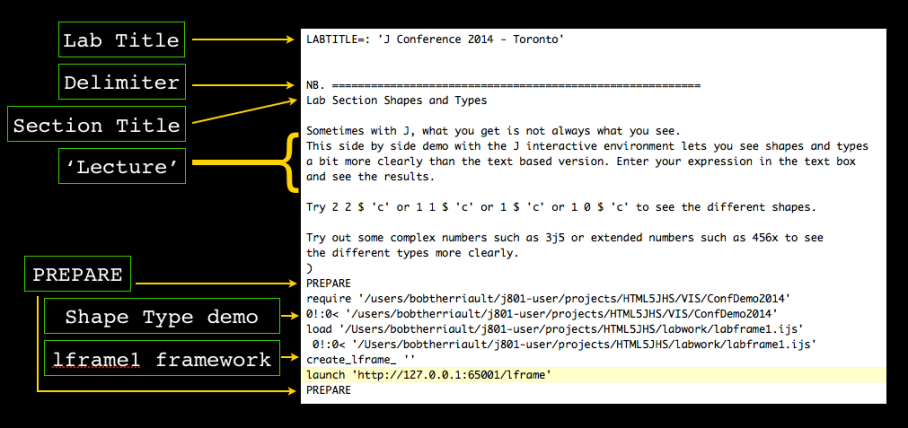
In the case of the example lab, ‘J conference 2014 – Toronto’, the PREPARE section launches the frame1 display which shows the jhs environment and an interactive display of shape and type side by side. frame1 is patterned on the demo9 example in the studio menu of the JHS environment, creating an html file with frames to display the different components.  The result is  two interactive frames side by side, with the jijx window displaying the ‘lecture’ for this particular lesson, in this case hints of phrases to enter.

BlogLab2

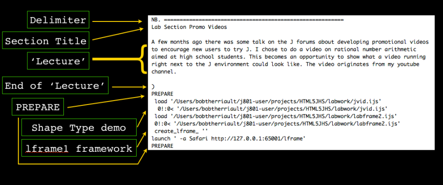
The second lesson launches frame2 but in that case a video replaces the shape and type demo. This video is the Ratio Arithmetic promo video that I produced and originates from my account in youtube. At this point only external videos may be run by the Safari browser. By using video animations and explanations of more complicated concepts combine to make for easier learning . At least that is the potential use, whether the combination of video, text and interaction works to make things clearer is down to the skills of the creator.


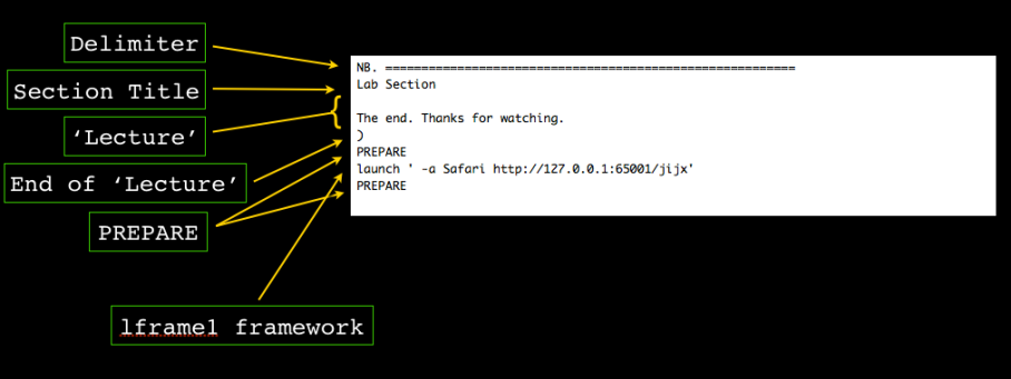
BlogLab3The final lesson returns back to the interactive jhs environment.

This will probably be as far as I will take this experiment with the lab framework, as Eric Iverson has suggested that it may be better to use the sp framework which has more capability for the new forms of interaction. The key thing I believe is to retain the structure of the lab files so that they are backward compatible and more importantly to potentially create a tool to allow easier creation of the augmented labs and at the same time enforcing lab structure with consistent results across platforms.

J Labs and why I find them so amazing.

Why Labs are Important

One of the most unique aspects of the J environment is the lab. Imagine that, a language with instructional support built in to the interface. Even more ambitious is that the support is provided not by page after page of description such as a man file in the unix system, – but by a series of  ‘lectures’ followed by access to the entire J environment to experiment on all those new ideas – and it is all just a menu click away in the standard J user interface.

How Labs are structured

Lab files all end with the .ijt extension and can be opened in any text editor. So how are these labs structured to provide this facility? The format of the lab files is simply a specifically formatted text file which the J environment, interprets and presents as a living lab. The file starts with some identifying header information and then moves into the main structure. Each time you advance the file you get some new information in a section of the lab. Most sections have two parts: 1)  a text message to the learner that ends with a single ‘)’ on its own line and 2) a series of executable J sentences and results that will be seen by the learner. Sections are combined to form chapters. the difference between sections and chapters is that J provides a way to jump between chapters but sections must be done in the same order each time. J labs can also do some hidden creation that the user does not see using the PREPARE keyword to bracket the section that will be executed invisibly. This allows the learner to focus on the lesson instead of developing the context of the lab. As a learner grappling with a new concept, the last thing you would want would be to perform a detailed series of instructions to create the results that you are trying to observe. This is also a reason that section need to be run in order because each lesson within the section may set up different parts of the environment and a misstep could result in very odd behaviour.

In conclusion

In a nutshell that is the mechanism behind the remarkable feature of the J language called labs. In future posts I will explore in greater depth the potential of labs when combined with HTML5 in the JHS environment and what approaches can be used to make these changes more effective. Eventually it would be good to create a tool that can easily create labs. I believe that it is by making the labs easier to create that we can actually involve more people in producing them and in that way develop an even more effective learning community for the J software language.

A short video to promote the J language

In response to work being done on the J forums in promoting J to various audiences, I decided to take aim at what I think would be a good audience for learning J – middle and high school math students. I kept the video short and focussed on the the utility of J’s use of ratio arithmetic.

If it looks as if this is on the right track, I have ideas on a few more of this style of video to raise the interest of newcomers to the J programming language.

An Update on Display Shapes and Types on JHS

Based on some consistent and clear comments from a number of J’ers I respect greatly, I have made some adjustments to the way that the HTML and CSS affect the display on JHS. Primarily I am not showing atoms as enclosed except for the case of literals where the blank spaces are important to the array display in ways that the numeric types are not. I instead use colour and font to distinguish between the types. In the case of shapes I really now only display the single and zero dimensions as a visible envelope around the atoms. This results in a much less noisy display.

I went into these changes thinking that this might be difficult to do, but found instead that by using CSS that a lot of the display changes are isolated from the structure that I have built using J to form the HTML. The script is available as an attachment to the page:

http://www.jsoftware.com/jwiki/BobTherriault/Visualize

under the name vlitejwiki.ijs

and below is a 3 minute video giving you an idea what to expect

Using CSS and HTML to display the shapes of arrays on the JHS platform

The following video will provide an idea of how HTML and CSS can be used to more clearly show the shapes of arrays on the JHS platform. This includes arrays with zero valued dimensions and arrays with single valued dimensions that would be displayed ambiguously in the text based format.

If you have not already viewed the preceding blog post on displaying different types of J variable, it may be worthwhile to take a look at it here. There is a brief review of types in this shape video but it does not cover the information in any great detail.

Using HTML and CSS to view Types in the JHS platform of J

Time flies when you are having fun, or maybe just time flies as I look back to how long it is since I have posted here. In any case I am back and ready to explore some new developments in the way that I am using the JHS platform of J.

One of the things that has frustrated me with J is that at times I spend a lot of time trying to figure out problems based on simple (and incorrect) assumptions I have about the information that I am being shown. J has an elegantly minimalistic way of showing the results of operations in its interactive environment. Unfortunately, it does not always distinguish between certain key qualities when it displays its results. It becomes my job as a programmer to confirm what I am seeing as what is really being presented and this is especially true for type information. With modern web browsers it has become possible to provide this additional information as part of the results and this is explored in the following video.

Since there was not enough time to go into all the details the screens below provide some of the background to the css and elements of html that are created in order to provide the new html based display. I provide this information for all to use and only ask that if you use it that in your best judgement you use it in a mindfully positive way.

Types

I hope to follow up in a week with the HTML and CSS approaches I have explored to display differently shaped arrays unambiguously, but last time I said that resulted in almost two years between posts. 🙂

Augmented View of Arrays (Redux)

Follow-up:

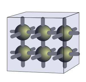
After looking back at the previous post I did notice one mistake. The shape for the following diagram should have been 1 2 3 instead of 2 3. If the shape had been 2 3 then the diagram would have had a plane rather than a cube as the ‘shape structure’.

 1 2 3 $ 0
Augmenting Frank’s Dual-View Representation by Simplifying:

After several weeks of reflection, I realized that the previous solution to visualizing Frank’s Dual-View could be made simpler  by displaying the absence of edges when there are zero valued dimensions in the shape. The following post will compare the two options with a following critique of the differences.

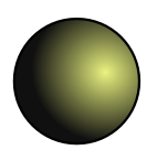
Case 0 – Empty shape for scalar value – Shape ’empty’


Old version
New version

Critique: The only difference here is colour to distinguish the two approaches as we move forward. Remember that scalar values in J do not have a shape of 0, but instead have a shape that is an empty list. Since there is no 0 in an empty list there is no change in representation of scalars.

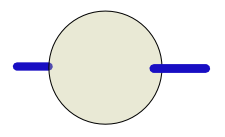
Case 1 – A list of zero items – Shape 0


Old version
New version

Critique: Both versions have the axle indicating that this is a list and that items can be added. Both versions are also greyed out as a visual cue that this is an empty list. The new version shows that the dimension that is zero is along the x axis (the only axis, as indicated by the axle) and so this is an empty list, as opposed to an empty matrix or cube which we will see later. Even though this adds an element in the visualization of an empty array, it will provide a more simple representation of non-empty arrays.

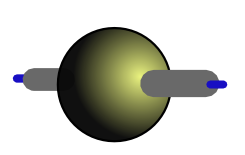
Case 2 – A list of one item – Shape 1


Old version
New version

Critique: This is where the advantage of the new approach starts to appear. Instead of the extra horizontal line, only the line presenting the one dimensional shape is included. The colour indicates that the shape is non-zero immediately.

Case 3 – A matrix of one item – Shape 1 1


Old version

New version
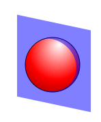
Critique: The advantage continues as the plane immediately indicates the two dimensional shape and the single sphere indicates only one item. No extra lines required for the vast majority of arrays which are non-empty.

Case 4 – A cube of one item – Shape 1 1 1


Old version
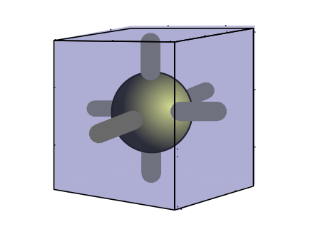
New version

Critique: Again we have a single atom and the surrounding cube indicates three dimensions. The extra edges in the previous version are not required which really cleans up the display

Case 5 – A matrix of one item – Shape 0, Shape 0 1, and Shape 1, 0


Shape 0

Shape 0 1

Shape 1 0

Critique: The displays of these three empty arrays show that the one dimensional and two dimensional are clearly distinguishable, as is the difference between Shape 0 1 and Shape 1 0 matrices.

Case 6 – A cube of shape 1 2 3


Old version

New version

Critique: The spacing of the spheres easily shows the shape of the array and the enclosing cube outline immediately shows that the array has a three dimensional shape. If it were two dimensions the spheres would be embedded in a two dimensional plane. Again no more and no less than what is required to differentiate and describe the shape.

Case 7 – A cube of shape 0 2 3

Critique: This one was thrown in to show how a zero value in the leading axis of a three dimensional array would look. There are two rows and three columns of zero items which is why the spheres are greyed out with a front facing zero mark on the z axis. Contrast this with the 1 2 3 shape described in the preceding example.

Case 8 – A cube of shape 2 2 3


Old version

New version

Critique: I think that I may want to play around with the spacing on this one as this is one case where the new representation actually seems more confusing than the old version. Part of it may be the inherent structure that the extra edges provide, but I think this can be made up by using the spacing to reveal the relationships between the spheres as rows and columns. The text version of J uses this spacing to great effect, so I feel I am moving the right direction even though this version feels relatively unorganized.

In closing:

This time I promise; the next post will look at the representation of higher ranked arrays. I was happy to spend the extra time revising the display, as the higher dimensional representations really benefit from the cleaner look.  Until next time, I look forward to any feedback you may have.