Augmenting the Dual-View Array Representation

Follow Up:

My previous post included a verb to facilitate visualization of the Dual-View representation by returning coefficients representing array components:

   arrayCoeff =: +//.@(*/)/@,.&1

Unfortunately, this verb fails for scalars because it can’t deal with the empty list shape of rank 0 arrays.

   arrayCoeff ''
|domain error: arrayCoeff
|       arrayCoeff ''

A better solution has the array itself as the argument, then determines its shape and triggers an exception when dealing with scalars.

   arrayCoeffS =: +//.@(*/)/@,.&1`1:@.(''&-:)@$

where

 (''&-: )@$

returns 1 for a scalar argument.

   arrayCoeffS 4  NB. Scalar, array rank 0, shape ''
1
   arrayCoeffS 3 $ 4 NB. Vector, array rank 1, shape 3
3 1
   arrayCoeffS 2 3 $ 4 NB. Matrix, array rank 2, shape 2 3
6 5 1

Augmenting Frank’s Dual-View Representation:

This will allow arrays of shape 0 and shape 0 1 to be shown as distinct.
The Dual-View shows these shapes as identical because rank 2 can’t be represented by a single edge.

   arrayCoeffS 0$0 NB. Empty list of rank 1
0 1 

   arrayCoeffS 0 1$0 NB. No list of length 1 (rank 2)
0 1 1

Clearly they differ in the rank 2 array’s planar component, and changing the orientation of the single edge to indicate the plane is identical to the result of:

   arrayCoeffS 1 0$0 NB. One list of length 0 (rank 2)
0 1 1 

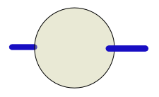
The way forward is to display the rank of the array even when the zero valued axes are not present. With distinguishable ranks, rank 1 and 2 arrays will be distinct. For rank 0 (scalar), the representation is the disk alone.

   arrayCoeffS 2 NB. Scalar value of 2 (rank 0)
1 

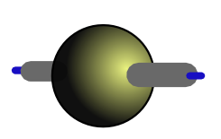
Arrays of rank 1 have a horizontal line through the disk indicating that the list can add items either before or after the value. If the shape is 0, only this rank line is shown with an empty value – a greyed out disk.

A non-zero axis uses thicker edges with rank line extended.

Rank 2 arrays indicate rank as an x-y plane encompassing the disk, allowing axes indication without affecting rank representation.

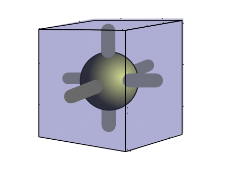
With rank 3 the embedding structure is a cube, with potential axes in three dimensions.

By including the rank information the augmented Dual-View shows previously indistinguishable arrays distinctly:

   0$0 

   0 1 $ 0 

   1 0 $ 0 

While typical arrays display as expected.

   2 3 $ 0 

   2 2 3 $ 0 

In the next post I will look at the representation of higher ranked arrays. Until then, I look forward to any feedback you may have.

The ‘Dual-View’ approach to array visualization

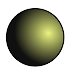
Previously, we found the J text representation revealed values of individual atoms, but could not distinguish singleton arrays of different shapes, or empty arrays. Ron Frank in his paper, “A New “Dual-View” Diagram of Array Structure” (Frank, 2003) describes “Dual-View”, applying combinatorics to enumerate the atoms, lists, planes and cubes and representing them with dots and edges.

For example, an array of shape 2 3 4 has 2 * 3 * 4 = 24 atoms (T00); (2*3)+(3*4)+(2*4)=26 edges (T01); 2 + 3 + 4 = 9 planes (T02); and 1 cube (T03).

Edges and dots indicate planes and cubes by sketching the array in three dimensions. Collinear segments count as only one edge, so the diagram above has 24 dots for atoms, 26 edges for lists (12 aligned vertically, eight horizontally, and six along the z axis), nine planes (two parallel to the x-z plane, four parallel to the x-y plane and three parallel to the y-z plane), in a three dimensional brick.

This monadic J verb produces these coefficients given the shape of the array by stitching 1 to items of the shape, then cross multiplying (2 1) ⊗ (3 1) ⊗ (4 1) to produce coefficients.

   arrayCoeff =: (+//.@(*/))/@,.&1 
   arrayCoeff 2 3 4
24 26 9 1

For single valued arrays the added edges create distinct representations.

   arrayCoeff 1
1 1

   arrayCoeff 1 1
1 2 1

   arrayCoeff 1 1 1
1 3 3 1

Empty arrays have at least one zero in their shape. The list with shape zero is represented by a single edge with no dot as predicted.

   arrayCoeff 0
0 1


For higher ranked arrays, edges indicate placement of planes and cubes.

   arrayCoeff 2 3 0
0 6 5 1

Above we see an array of shape 2 3 0 with two planes parallel to the z-x plane (two pairs of three edges) and three planes parallel to the z-y plane (three groups of two).This representation conveys the empty array of shape 2 3 0 distinctly. A previous post illustrated that distinct orientations can represent shape permutations.

When more than one item in the shape is zero, for example shape 0 2 0, difficulties with the “Dual-View” crop up.

   arrayCoeff 0 2 0
0 0 2 1

As before we have zero atoms, but we also have zero edges – an invisible representation, making it impossible to distinguish arrays with more than one zero in their shape. In the next blog post I’ll introduce augmentations to the “Dual-View”, and although this improves the representation of array shapes, I must say the J text representation remains best for showing values of atoms.

References:

Frank, Ronald I. (2003). A New ‘Dual View’ Diagram of Array Structure,
Proceedings of the ACM APL (SIGAPL), Federated Computer Research Conference (October 2003). ISBN 1 58113 668 4.

Singletons and Wide Open Spaces

In good representations, similar things will look alike and distinct things will look different. In great representations, good representations combine with metaphor to create meaning. The metaphor used in J is the array. If you are not sure of J’s approach to rank, shape, or item then take a look at the previous post, otherwise let’s dive right into the spot that the J text representation breaks down. If we have an array with rank 1 and shape 1, it would look like this:

   A1=: 1 $ 4
   A1

4

And if we had an array with rank 2 and shape 1 1:

   A11=: 1 1 $ 4
   A11

4

And if we had an array with rank 3 and shape 1 1 1, it would look like this:

   A111=: 1 1 1 $ 4
   A111

4

Now using the “Shape Of” monadic verb ($) it is easy to get the shape information we want:

   $ A1

1
   $ A11

1 1
   $ A111

1 1 1

But if we only consider the representation, we find that things that are different look the same, which is a problem. Taking it one step further, let’s look at an atom. This particular atom is an integer:

   A=: 4
   A

4
   $ A


Atoms are arrays with an empty shape, and in this representation they look like other singleton arrays. The empty line represents the atom’s empty shape, but as innovative as this approach is, we still can’t discern single value arrays from atoms or one another.

To be fair, it is not only the J representation that has this problem. Looking at the block representation:

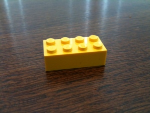
Single lego block

We notice that a single block could be a list of shape 1, or a table of shape 1 1, or a brick of shape 1 1 1. In fact, we are even at a bigger disadvantage with the block representation because an atom such as A would look like this:

No lego blocks

Or maybe perhaps the atom would be colour without the block, since the block has an empty shape. At least J can show us the value of the atom.

The second area where the J representation breaks down is how it shows empty arrays. An empty array is an array that has a zero (sometimes more than one) within its shape. If we create an empty array of shape 0 we’ll see the challenge of representation:

   A0=: 0 $ 2
   A0


   $ A0

0

which means that A0 displays as an empty line (a list with 0 length), and the shape of A0 is 0. This is a good representation as far as it goes, but it gets complicated with rank 2 arrays:

   A00=: 0 0 $ 2
   A00
   $ A00

0 0

Here, the shape 0 0 means no lists of length 0 and the empty line disappears. This suggests a difference between arrays of shape 0 and shape 0 0 which is good, but when we look at an array of shape 1 0, our one empty line returns:

   A10=: 1 0 $ 2
   A10

   $ A10

1 0

But an array of shape 0 1 looks identical to an array of shape 0 0:

   A01=: 0 1 $ 2
   A01
   $ A01

0 1

And if we think the problem is with J’s text limitations, with physical objects, representing empty arrays becomes quite impossible. We could make a zen koan about showing the shapes of things that are not there, but it would still not make the representation any clearer.

No lego blocks

In the last two blog posts we have developed language to describe arrays, and used that language to show the problems with both J’s text representation and a block representation. The next post will be about a visualization method which solves some of these array representation problems. In the meantime, any response that you have is welcome; either about the presentation style for these ideas or regarding the ideas themselves.

Looking at Arrays

In good representations, similar things will look alike and distinct things will look different. In great representations, good representations combine with metaphor to create meaning. The metaphor used in J is the array. If you are aware of J’s approach to rank, shape, or item then skip ahead to the next blog entry, otherwise read on.

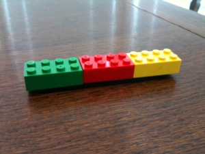
Row of three lego blocks

Here we have three blocks in a row. This array has three items and its shape is 3.

Using the J text representation we’d show it this way:

   A3=: 3 $ 5 6 7

where $ is the dyadic verb “Shape” that takes the right argument and makes it into the shape specified by the left argument. The =: is the assignment operator that assigns the result to the variable we have called A3:

   A3

5 6 7

We have A3 representing three numbers in an array (list) of shape 3. J can tell us this using the monadic form of $ known as “Shape Of”:

   $ A3

3

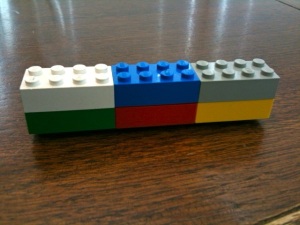
Two rows of three lego blocks

This one has two rows of three blocks suggesting that the shape is 2 3. We could also think of this array as two items, where each item is a row of three blocks. The same array in J would look like this:

   A23=: 2 3 $ 5 6 7 8 9 10
   A23
 
5 6 7
 
8 9 10
   $ A23

2 3

In J is the number of items in an array is the first item in the shape (yes the shape is an array as well and it has items). J uses the monadic verb “Tally” (#) to return the number of items in an array:

   $ A3

3
   # A3

3
   $ A23

2 3
   # A23

2

A big difference between the shapes of A3 and A23 is that the shape of A3 has 1 item and the shape of A23 has 2 items. This idea of the number of items in the shape is interesting enough that we give it its own name: rank. So A3 has rank 1 and A23 has rank 2. In J we can find this by using the monadic verb # “Tally” to find the number of items in the shape, like this:

   # $ A3

1
   # $ A23

2

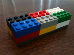
Two planes each with two rows of three lego blocks

Above, we have a brick of 2 tables, each table with 2 lists, and each list with length 3. Using J we get:

   A223=: 2 2 3 $ 5 6 7 8 9 10 11 12 13 14 15 16
   A223
 
5  6  7
 
8  9 10


11 12 13

14 15 16

and:

   $ A223

2 2 3
   # $ a223

3 

Using the empty line to separate each item in the array is a particularly clever approach that J uses to display higher rank arrays. In fact, J adds an extra line as the rank increases, so that the items in rank 4 arrays are separated by 2 empty lines.

To sum up: (1) arrays have shapes, (2) the first number in the shape is the number of items, (3) the rank of an array is the length of its shape. If this isn’t clear, go back and review the examples above or take a look at Chapter 5 in Henry Rich’s excellent “J for C Programmers”. In the next blog entry we’ll explore why the J representation for arrays is not as clear as it could be.

Block Representations of J’s arrays

When I moved to a house on the edge of a forest I enjoyed many hours exploring the trails, but when maps placed at strategic points consistently sent me in the wrong direction, I thought years away from the world of compass points and orienteering had finally caught up with me. It was not until I stood looking at a map in front of Enos Lake that I discovered the real reason. The map suggested that the lake, which was clearly before me, should in fact be located behind; the map had been mounted backwards with respect to the surrounding terrain. As I saw more maps on the trails, I found that they had all been placed with a similar aspect; even more misleading because they were usually in the middle of the forest, away from prominent features that allowed reorientation.

And the point of this story? Well for the last couple of years I have considered translating the textual form of the J computer language into a visual one, and it has become clear that visual interpretation requires coordination with the structure of the language on a fundamental level. As with my experiences on the trail, it is vital that the map (visual interface) fit the terrain (the structure of the language), or at every step along the way we risk losing our users due to unnecessary mental effort.

So let’s look at the J’s terrain before we position our map. J uses a text based representation to expresse values and structures of its arrays to the programmer. While this style is very good at showing the values of the arrays, it is less effective in conveying their shape and structure (particularly in the case of singletons or arrays with zero valued indices in their shape). For now let’s look at how an array of 2 numbers would be shown.

       2 $ 1 2
1 2

To explain, the top line is the instruction to create the array and the second line is the representation. On the top line, the 2 in front of the $ means that the 2 items after the $ will be used to make an array of length 2.

If we represented the numbers as children’s blocks it might look like this:

Similarly a two-dimensional array would be represented with rows and columns. In the example below there are now two numbers before the $. The first number, 3, gives the number of rows and the second number, 2, gives the number of items in each row.

      3 2 $ 1 2 3 4 5 6
1 2
3 4
5 6

And in block notation we could stack the blocks as follows:

When we move to three dimensions it gets a bit more complicated. There are now three numbers before the $, and the first number, 3, indicates the number of 3 X 2 planes that we will have. J uses the linefeed to insert an empty line between the planes and separate them in a very effective way.

     3 3 2 $ 1 2 3 4 5 6 7 8 9 10 11 12 13 14 15 16 17 18
 1  2 
 3  4
 5  6 

 7  8
 9 10
11 12 

13 14
15 16
17 18

If we use the blocks, the situation presents a choice that was not present in our first two examples. Do we stack the planes with the first plane at the back or at the front? Here is an example of the two approaches:

Either choice could work but I prefer having the planes stack like the pages of a book, with the ones closest being the ones that are listed first. This also allows the position in the upper left front corner to be an anchor easily located by the viewer. If instead the planes were added moving forward toward the viewer, then the visible corner value would change as every plane is added. There are enough challenges in understanding array languages without having the positions in the array dance before your eyes.

And it is at this point, gentle reader, that you come in. My perception is but one data point in creating representations for a much wider audience. I welcome feedback about the suitability of the ‘book pages’ approach to three-dimensional arrays, but concerns about the row and plane representations in the case of two-dimensional arrays are important as well in revealing even deeper fundamental differences in visualization. Don’t worry about the fact that J’s text approach and my block visualizations do a poor job of distinguishing between atoms, lists, or matrices of only one value, I will be addressing that in a future post. For now, just let me know if the direction my map is pointed makes sense to you.

Thanks in advance for your help.

Video Annotation for Lesson 4 of Idiosyncratic Introduction

Here is the new video annotation for the fourth lesson of the Idiosyncratic Introduction to J. The changes in approach in this video are most visible about half way through where I make some changes to accommodate the challenge of displaying matrix operations. In the end I opted to use an ‘in-place’ method using highlights to indicate the argument to the operator. I like this enough that in the end I may make some reversions to the earlier labs to make them consistent, but obviously before I do I would love wider feedback on the new video.

The new version of Lesson 3 Video Annotation

This is a new version of the Lesson 3 video annotation based on a suggestion by Raul Miller. Raul’s concern was that the previous version had too busy an animation. Why not do the operation across lists vertically by layering the lists instead of rotating from horizontal to vertical and back again. The advantages of this is that the animation is cleaner and quicker and the use of the assignment operator (=.) is not required. The challenge is that left argument mus be above the right argument for non-symmetrical operators such as Minus (-) and Divides (%) and the spacing of the columns depends on the width of the results. Let me know whether this version is an improvement. I look forward to your feedback/comments.

Cheers, bob

Video for Lesson 3 of Idiosyncratic Introduction to J

Well at least it did not take as long to get the video for Lesson 3 up and running. I took a slightly different approach here and animated the actual lines of J to show how the calculations take place. This is pretty straightforward for lists/vectors but may become more complicated when 2 dimensional arguments are used in the next lesson. I may need to draw on my experience with some of the NuVoc videos … and then again I may come up with something different again.

As always, comments and suggestions are welcome.

Cheers, bob

You ain’t heard nothing yet

Yeah, I know it has been a while and you have every right to be concerned about the pace of this project – I know I have been at times. But what you don’t get a chance to experience is the amount of behind the scenes development that has gone on.

For one thing, it turns out there is a very nice way to add sound to Keynote animations – that’s good – and it also turns out that the reliability of Keynote timing when exporting to video is suspect – frustrating. As a result, the Keynote animations need to be moved to iMovie, have the voice over added and timed out to result in a reliable video output. The result is actually more efficiently produced – more updates to follow – and allows exact timing of voice over and animation – vital.

Here is the Lesson 2 annotation to “An Idiosyncratic Introduction to J” by Roger Hui.

Video Annotation for Lesson 2 of An Idiosyncratic Introduction to J

First, an admission that these videos do take a while to produce and in the process of developing them I am still discovering the most efficient workflow and optimal tool use. So, if you think that the only productive area is the final result, remember that there is much work going on behind the scenes.

This video involves much more animation than the first one and I think it hints at the power that these annotations can have as we move forward into lessons that have more cognitive challenges.

For now, watch this one and let me know whether the process is working for you as a viewer. If it isn’t, please let me know (extra special bonus points if you can also suggest a solution, but just pointing out the issue is sufficient).

Cheers, bob